|
|
||||||
|
|

May 6, 2013 Aligning Market Exposure With the Expected Return/Risk Profile Some risks and market conditions are more rewarding than others. My objectives for this week’s comment are very specific. First, to demonstrate – using a very simple model – that investment returns do indeed vary systematically with market conditions. Second, to demonstrate that overvalued, overbought, overbullish conditions have historically dominated trend-following measures when they have emerged. Third, to demonstrate the impact of accepting investment exposure in proportion to the return/risk profile (technically the “Sharpe ratio”) that is associated with a given set of market conditions. My hope is to walk through the general framework of how I think about market exposure. However, what follows is not a description of the investment models we use in practice, which involve more numerous considerations and a much broader ensemble of models and methods. The measures I present here are very simple, and while even these conditions identify strong distinctions between market conditions, they are nowhere close to the degree of separation that can be obtained and validated across history with a broader ensemble of evidence. The discussion here will not help to understand my “miss” in 2009-early 2010, which was related to the need to stress-test our approach to ensure that it was robust even to the worst portions of Depression-era data. It’s incorrect to view that “miss” as a result of our indicators, strategies, or valuation methods; it resulted from the similarity between Depression-era events and what the U.S. economy was actually experiencing in real-time, and my insistence on having the a robust method to navigate that uncertainty (despite our existing methods doing just fine to that point). Both trend-following methods and typical valuation thresholds were torn to pieces during the Depression, far more violently than investors may appreciate. Like me or hate me for that decision, but I wouldn’t fly a plane that I wasn’t certain could handle extreme turbulence – and I expect there will be more of that turbulence over the coming decade than investors seem to envision here. A practical note – as of Friday, our estimate of prospective 10-year S&P 500 total returns (nominal) has dropped to just 3.3%. With the exception of 1929, this level of estimated returns was never observed in historical data prior to the late-1990’s market bubble. Rich valuation is not a rally-stopper in itself, and we’ve certainly narrowed our defensive criteria enough to entertain a more constructive stance under some conditions without a steep market decline first. But the end-game here is still most likely a 30-50% market decline over the next 2-3 years, which would be far more than enough to wipe out any interim market gains. To dismiss that likelihood is to ignore predictable experience since 2000, as the bubble-bust cycle of easy money has repeatedly interacted with rich valuations to produce gleeful roller-coaster rides with very bad endings. Again, my objective here is to detail my general approach to thinking about market exposure, which is the best way to understand my present views, and what one can expect going forward. There are certainly portions of the recent market cycle (particularly that 2009-early 2010 period) where even this simple model was more effective in hindsight than the “first-do-no-harm” approach that I insisted on once the credit crisis forced us to contemplate Depression-era outcomes. The advancing half of the present, unfinished market cycle began with that stress-testing episode, and since 2010 has continually demanded research into how long a frog can or should remain in a heated cauldron without ending up dead in the water. Refinements based on trend-following and momentum measures, under certain conditions, can help to more finely navigate the late-stage, overvalued portion of a bull market and avoid an overly early exit. Strategically, none of that is actually required to do well over the complete market cycle, but I would obviously have had an easier time with QE in recent years had I allowed the frog to break into sweat and hallucinations before yanking him out of the kettle. He’s quite willing to plunge in, or at least dangle his little legs into the water, as opportunities arise. I expect the effect of all that to be evident over time. Staying Sharpe We’ll start with two useful concepts. One is sometimes called the “excess return” of the market, which is the total return of the S&P 500 in excess of Treasury bill yields. A negative expected excess return means that stocks are expected to underperform the risk-free alternative. A positive expected excess return means that stocks are expected to outperform the risk-free alternative. Clearly, we should prefer to accept risk only when we expect to be paid, on average, for doing so. The second concept extends the idea of “excess return” by measuring that return per unit of risk. The “Sharpe ratio” essentially takes the expected excess return and divides it by the expected risk (measured as volatility or standard deviation). We should prefer to accept more units of risk when we expect that risk to be compensated by a strong excess return (this is particularly true if we have a “risk budget”). In fact, nearly every “dynamic portfolio allocation” model in the literature of finance has this central feature: the optimal investment exposure is proportional to the excess return per unit of risk that can be expected at each point in time. While some continuous time models – like those of Merton and Samuelson – sometimes include additional “hedging demand” that relates to how prices vary as expected returns change over time, the core structure of nearly all optimal portfolio allocation models is that investment exposure should be relatively proportional to the excess return that can be expected per unit of risk. [Geek’s Note: if you solve the dynamic optimization problem, you actually get an investment demand function where the denominator is a risk-aversion coefficient multiplied by the variance of returns rather than the standard deviation. But given that variance is much more stable than expected return, there’s little impact to subsuming one of those sigmas into the risk-aversion coefficient and varying exposure in proportion to the expected Sharpe ratio. An extra “hedging” term is necessary for models that use a long-term prospective return in computing the Sharpe ratio, as the correlation between that prospective return and realized returns is significantly negative. “Hedging” in this context means hedging against changes in the investment opportunity set. That correlation is negligible for the version that we’re discussing here, which is based on instantaneous expected returns]. What really differentiates investment approaches (or at least, what ought to differentiate them) is the approach that is used to estimate that expected return/risk profile. Though my insistence on getting this right in the face of potential Depression-type outcomes did us no favors in the unfinished half of this particular market cycle, a robust approach to estimating return/risk profiles, and the discipline to consistently maintain alignment with them, are the most important tools in asset allocation. For expositional approaches (only), we’ll use a relatively simple model to demonstrate these concepts. Let’s start with one of the most common trend-following approaches, which is to track the market’s position relative to a moving-average on the order of about 10 months, 200 days, or 39 weeks. Below, we’ll use a 39-week smoothing. Since 1940, when the S&P 500 was above its 39-week smoothing, the total return on the index, in excess of Treasury bills, has averaged about 9.6% annually. In contrast, when the S&P 500 was below its 39-week smoothing, the excess return averaged just 0.3% annually. It’s interesting that since early 2010, a switching strategy based on this fact would only be up about 8.3%, and transaction costs and slippage would have eaten up much of that. Still, there’s no question that trend-following components are extremely useful in any full-cycle investment approach (particularly for loss reduction). Interestingly, even when trend-following measures are favorable, the market has historically not performed well when overvalued, overbullish conditions have also been in place. Let’s define these very simply here – say a Shiller P/E greater than 18 (the ratio of the S&P 500 to the 10-year average of inflation-adjusted earnings), and advisory sentiment featuring more than 47% bulls and less than 27% bears at any point over the most recent 4-week period (based on Investors Intelligence figures and imputed prior to the 1960’s). Historically, this combination of conditions has been associated with an average excess return of -4.6% at an annual rate, and -4.2% even when the trend has been positive. Meanwhile, valuations have also been extremely useful in distinguishing strong Sharpe ratios from poor ones. Again, for simplicity, let’s use a Shiller P/E of 18 as a threshold. Since 1940, periods with the S&P 500 above its 39-week smoothing and the Shiller P/E below 18 have been associated with total returns in excess of T-bills averaging 15.1% at an annual rate. Periods featuring neither have been associated with total excess returns averaging -1.9%. Periods with the S&P 500 below its 39-week smoothing and the Shiller P/E below 18 are typically quite volatile, and average a 1.2% average excess return. The fourth possibility is the interesting one at present. While periods with the S&P 500 above its 39-week smoothing and a Shiller P/E above 18 (it’s presently approaching 23.7) have averaged an excess return of about 4.3% at an annual rate, all of that return actually loads onto periods where overbullish conditions were absent. If we look at the combination with favorable trends and overvaluation but an absence of overbullish conditions, the excess return has averaged 11.7%. In contrast, when overbullish conditions have been in place, the overvalued, overbullish conditions have dominated, producing a negative excess return averaging -3.3%. The following is a summary of some of these simple investment environments and their historical frequencies in data since 1940 (not all of them are mutually exclusive). SPX = S&P 500, MA = MA39, OVOB = overvalued, overbullish, PE = Shiller P/E ratio.
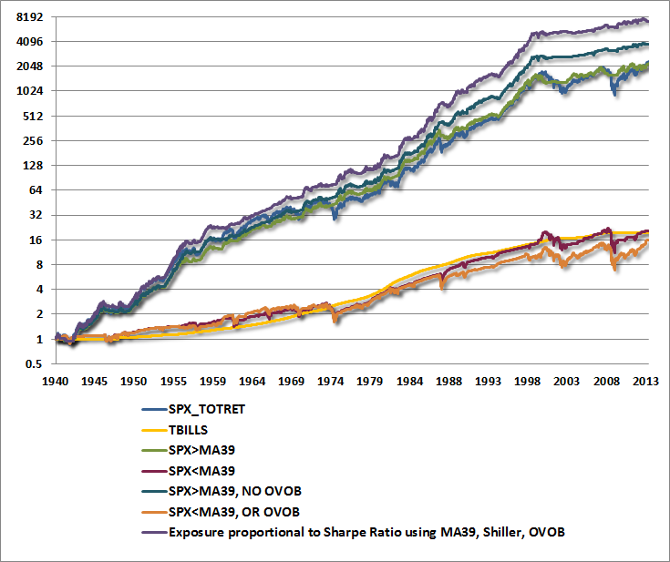
I should note that in practice, it’s essential that estimates of expected excess returns and Sharpe ratios should be validated in multiple split samples across history, as well as holdout data that was not “seen” at all by the estimation approach. For the conditions I’ve noted above, all of these separations do hold up in split samples, but again, my intent here is to demonstrate a very basic model. This model is far simpler and less effective than the ensemble approach that actually informs my views, it doesn’t reflect transaction costs or slippage, and it does not reflect the strong validation considerations required of a real-world approach. The chart below shows a switching strategy (holding T-bills when out of the S&P 500) where exposures are taken in proportion to the Sharpe ratio, allowing a slight amount of leverage where the Sharpe ratio exceeds 1.0 on an annual measure, and slight short positions where the Sharpe ratio is negative. Notice that most of the market’s historical gains are captured in periods where the S&P 500 has been above its 39-week smoothing (MA39). Switching does a reasonable job of risk reduction, but it is still subject to significant drawdowns periodically (particularly in Depression-era data). Not surprisingly, excluding overvalued, overbought periods (OVOB) has performed better. The strongest approach over complete market cycles and over history, again not surprisingly, has been to align investment exposure with the prospective return/risk profile based on conditions at each point in time. The version below uses the combination of MA39 and Shiller P/E, except when MA39 is positive and the Shiller P/E is over 18, in which case, OVOB is used to further partition market conditions.
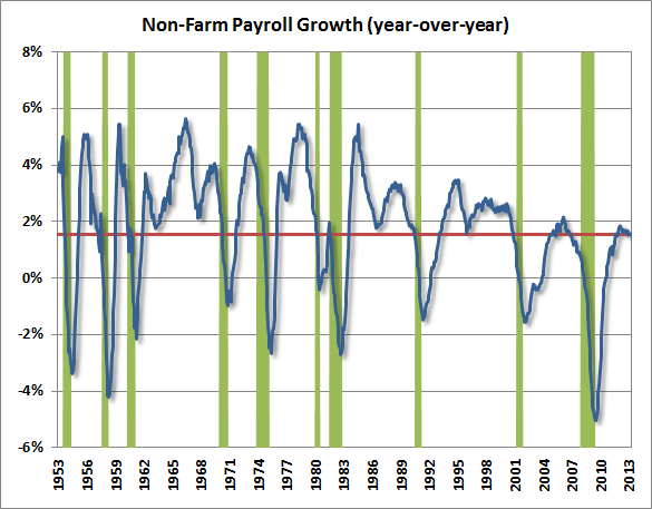
A few observations – again, these figures are hypothetical and don’t reflect transaction costs, slippage or other factors, but do provide some insightful context. Measured from the 1990 market peak to the 2000 market peak, the S&P 500 gained about 432% overall, including dividends. MA39 gained 262%, MA39 without OVOB gained 362%, and the Sharpe Ratio approach gained 394%. It was very difficult for any strategy to outperform a straight buy-and-hold during the bubble. But notably, measuring the full cycle from the 1990 market trough to the 2002 market trough, the S&P 500 gained just 245% overall, MA39 gained 262%, MA39 without OVOB gained 373%, and the Sharpe Ratio approach gained 444%. The deepest drawdown losses were 46% for the S&P 500, 23% for MA39, and less than 15% for MA39 without OVOB and the Sharpe Ratio approach. In the 2000-2007 peak-to-peak cycle, the S&P 500 gained 16% including dividends, with a 46% interim loss (weekly data), MA39 gained 41% with a 23% interim loss, MA39 without OVOB gained 22% with an 8% interim loss, and the Sharpe Ratio approach gained 18% with a 9% interim loss. Measured from the 2002 trough to the 2009 trough, the S&P 500 lost 3% overall after a 55% drawdown, while each of the other strategies gained more than 10%, with the worst drawdown for MA39 at 21%, and smaller losses for the others. Notably, the deepest loss for the Sharpe ratio strategy in weekly data since 1940 was just over 18%. Measured from the 2007 peak to the present, all of the strategies have roughly matched the S&P 500, with the deepest interim drawdown for MA39. What’s striking though is that all of the strategies have badly lagged the S&P 500 since April 2010, with returns of less than 10% each. This is true even for a pure trend-following strategy using the 39-week smoothing. Part of the reason for this is the degree to which market returns in recent years have come in the form of vertical spikes in response to sudden monetary policy announcements, just after trend-following approaches were whipsawed into a defensive position by the preceding market decline. The questions here are these. Given that a buy-and-hold approach has outperformed these other strategies in recent years, should we assume that aligning investment exposure with prospective return/risk is no longer a useful approach? Should we assume that the market has achieved a permanently high plateau, or better – a permanently upward diagonal – and that downside risk has been eliminated? Should we assume that the failure of risk-managed strategies to match the performance of a speculative ramp in prices (as they did leading up to the 2000 market peak) will continue indefinitely, and that risk-managed approaches should be abandoned out of faith in a central bank that has repeatedly demonstrated its capacity to produce bubbles that ultimately collapse? In my view, the introduction of quantitative easing and the expansion of fiscal deficits does not repeal market cycles or make risk considerations irrelevant. They certainly should not encourage investors to depart from the principle of aligning their exposure to market risk with objective estimates of how such exposure is likely to be rewarded or punished. Long-term investment returns typically emerge as the delayed payment for adhering to a sound discipline even when it is uncomfortable to do so. Immediate investment returns are often easier to find, but they tend to be advances on a loan that will eventually be repaid with interest. There is no question that new features of the market environment, when observed, should be examined for their interaction with existing features. But it has never been the case that these new features have served as a veto against all other considerations. It wasn’t true of the dot-com and tech bubble. It wasn’t true of the housing bubble. It is not true of the QE bubble that the Fed has created today (and which is overlooked primarily because corporate profit margins are 70% above historical norms as a result of mirror-image deficits in the combined government and household sectors – not just domestically but globally). Investment exposure should be aligned with the estimated return that can be expected in return for the risk one accepts. It is clear that market returns do indeed vary depending on observable conditions, and although returns can certainly depart from expectations during various portions of the market cycle, there is a century of evidence to support the proposition that this kind of disciplined investment allocation has been effective over complete market cycles, and has significantly reduced the depth of periodic losses. Economic Notes It’s worth observing that despite the modest but legitimate surprise in April employment, year-over-year growth in non-farm payrolls has now dropped below 1.6% for the second month; something that is typically observed only during or prior to recessions (shaded in the graph below). Real GDP and real final sales also both slowed to their typical pre-recession thresholds (1.8%) in first quarter data. This instance may be different, and repeated bouts of monetary easing have certainly kicked the can repeatedly with some success. Still, in light of the nearly unanimous deterioration in regional purchasing managers surveys, with no material strength in Philly Fed or the new orders component of the Chicago Purchasing Managers survey (two of the better leading measures), it’s difficult to share the enthusiasm that a modest beat on a lagging economic indicator signals a new economic Renaissance.
The foregoing comments represent the general investment analysis and economic views of the Advisor, and are provided solely for the purpose of information, instruction and discourse. Only comments in the Fund Notes section relate specifically to the Hussman Funds and the investment positions of the Funds. Fund Notes As of last week, market conditions continued to be characterized by overvalued, overbought, overbullish features that have historically been hostile to stocks. Over the past few years, we have worked to narrow the set of market conditions that warrant a defensive position – essentially to identify observable factors that help to refine the pool of outcomes to the most negative instances, and to thereby free the other instances from a defensive position. This sort of “exclusion analysis" can be very useful. Suppose for example that we write the number -10 on five pieces of paper, and +2 on ten others. The average value on those fifteen pieces of paper will be -2. But if we can exclude five pieces with +2 on them, we can concentrate our attention on the smaller set of more pointed outcomes (now ten with an average value of -4), and free up the remaining ones. As a practical example, even when our ensemble approach has indicated a negative expected return/risk tradeoff on the basis of a broad range of market conditions, it turns out that the worst outcomes are heavily concentrated in periods where either our best trend-following measures are negative, or when overvalued, overbought, overbullish conditions have emerged. As I noted in early 2012, points where the trend-following measures are positive and overvalued, overbought, overbullish conditions are absent could be “freed” from strongly defensive positions despite a negative return/risk estimate. That would have made certain points in 2010 and 2011 more comfortable by reducing the frequency of our most defensive positions. Recently, we have allowed the market to advance without equally raising our “staggered strike” position in Strategic Growth Fund. A staggered-strike hedge raises the strike prices of the index put option side of our hedge, and has historically been indicated about 5% of the time in data since 1940, based on a significantly negative expected return/risk profile at those points. A careful "exclusion analysis" suggests waiting until a flattening of momentum is observed before moving those strikes higher - they are presently about 4-5% below market levels. Note that we are now talking not about just the trend (the "first derivative") but the momentum (the "second deriviative") of the market. Most trend-following triggers such as standard moving averages are too distant to provide much loss avoidance, so momentum has become the one remaining criterion we can find (and validate) to separate a small percentage of benign short-term outcomes from a larger set of dismal ones. This sort of subtlety is not at all required over the course of the complete market cycle, but it may help to reduce some short-term discomfort if the market continues to advance (which I doubt, but can't rule out in any single instance). In an environment where euphoria begs investors to accept risk on blind and short-term speculative faith, much of my research effort is centered on every way possible to help investors maintain an informed and full-cycle discipline. We will be thrilled when conditions indicate a strong expected return/risk tradeoff. Those are not the conditons we presently observe. Our investment discipline remains focused on accepting market risk in proportion to the return that we expect to be associated with that risk, on average. In effect, within certain investment restrictions, we are looking to accept risk in proportion to the expected Sharpe ratio (defined as the expected market return in excess of Treasury bills, divided by the volatility of those returns). Investors who follow other disciplined investment approaches are often implicitly doing the same thing. Consider a disciplined trend-following approach, for example. Since 1940, when the S&P 500 has been above its 39-week moving average, the annualized total return of the index has averaged about 9.6% above Treasury bill returns (a Sharpe ratio of 0.78). The index has averaged just 0.3% when it has been below its 39-week average (a Sharpe ratio of 0.01). An investor who buys the S&P 500 above the moving average and exits the market below that moving average is essentially taking a position in proportion to the expected Sharpe ratio, where the factor of proportionality is 1.28 (that is, 1.28 x 0.78 = 100%). That’s not an endorsement of this strategy, and I believe that overvalued, overbought, overbullish considerations dominate trend-following ones here, but hopefully this example explains the concept, which I view as central to disciplined investing. As a side note, I suspect that it is not well-known that in data since 1940, the return/risk estimates from our present ensemble approach would have supported the use of leverage (a fully invested and unhedged position, with a few percent of assets in call options) in about 51% of historical periods, and zero or minimal hedging in another 10% of historical periods. A significant market exposure is reasonable in periods that are associated with a similarly positive expected Sharpe ratio for the S&P 500. By contrast, a significantly or fully hedged position would have been supported about 34% of the time (conditions associated with a negative Sharpe ratio), while a hard-defensive position such as a staggered-strike hedge was indicated in only about 5% of the data (conditions associated with a severely negative Sharpe ratio). Even when the expected Sharpe ratio of the market is severely negative, a staggered-strike hedge using higher strike put options is our most defensive stance in practice. There’s certainly no assurance that the same conditions will be associated with equally disparate market outcomes in the future, but these figures should give some indication of the frequency of investment positions I would expect under reasonably normal circumstances. These frequencies should also give an indication of how strikingly extreme and out-of-character recent market conditions have been from a historical perspective. I recognize that my legitimately unfortunate "miss" in 2009-early 2010 (I insisted on making our approach robust to Depression-era outcomes, which appeared largely indistinguishable from real-time), coupled with my intentional, evidence-driven defensiveness in recent years, and then blended with my successful anticipation of the 2000-2002 and 2007-2009 declines, has given me the reputation of a permabear. Keep in mind that the 2000-2002 decline wiped out the entire total return of the S&P 500 in excess of T-bills, all the way back to May 1996. The 2007-2009 decline wiped out the entire total return of the S&P 500 in excess of T-bills, all the way back to June 1995. Years, and years, and years of investment returns can be all for naught when investors forget that markets move in cycles. Frankly, it might be more scathing to be called a “permabear” if the period in question did not represent a 13-year span in which the S&P 500 has achieved a total return of just 2.3% annually, with two separate 50% market plunges, both of which I anticipated in vivid detail, and most likely with another market loss on that order that I expect will complete the present cycle. Still, we do not require anything close to such a market loss to support a more constructive position. We do require a positive expected Sharpe ratio, but the conditions associated with that are historically more varied and plentiful than one finds at the highs of an unfinished half-cycle. To everything, there is a season. Strategic Growth Fund remains fully hedged, with a staggered-strike hedge representing less than half of a percent in additional time premium (compared with a matched-strike long put/short call hedge). Those strike prices may be raised further in the event we observe a flattening of upward momentum. For now, the majority of day-to-day fluctuation in the Fund can be expected to reflect differences in performance between the stocks held by the Fund and the indices we use to hedge. Strategic International remains fully hedged. Strategic Dividend Value is hedged at about 50% of the value of its stock holdings. Strategic Total Return continues to carry a duration of about 3 years (meaning that a 100 basis point move in interest rates would be expected to impact the Fund by about 3% on the basis of bond price fluctuations). Based on a variety of factors, our return/risk estimates in precious metals shares backed off modestly last week, and we clipped our exposure to a smaller but still constructive 14% of assets. --- The foregoing comments represent the general investment analysis and economic views of the Advisor, and are provided solely for the purpose of information, instruction and discourse. Prospectuses for the Hussman Strategic Growth Fund, the Hussman Strategic Total Return Fund, the Hussman Strategic International Fund, and the Hussman Strategic Dividend Value Fund, as well as Fund reports and other information, are available by clicking "The Funds" menu button from any page of this website. |
|||||||||||||||||||||||||||||||||||||||||||||||||||||||||||||||||||||
|
For more information about investing in the Hussman Funds, please call us at
1-800-HUSSMAN (1-800-487-7626) 513-326-3551 outside the United States Site and site contents © copyright Hussman Funds. Brief quotations including attribution and a direct link to this site (www.hussmanfunds.com) are authorized. All other rights reserved and actively enforced. Extensive or unattributed reproduction of text or research findings are violations of copyright law. Site design by 1WebsiteDesigners. |